Embers by Example
The primary use case for EMBERS is the analysis of Radio Data obtained during the measurement of MWA antenna beam-patterns using satellites. The following examples outline the pipline used in the analysis of data for the Paper [Coming soon].
Setup
EMBERS works best in a virtual environment and requires Python > 3.6. Follow the Installation Instructions to setup a suitable enviroment.
$ mkdir ~/EMBERS
$ cd ~/EMBERS
The above creates an EMBERS directory, within which we can run our example code. Outputs will by default, be saved to ~/EMBERS/embers_out.
Alternately, for an directory in an arbitrary location /foobar/EMBERS, outputs will be saved to /foobar/EMBERS/embers_out.
We now download sample data required to run the subsequent examples from the EMBERS Sample Data github repository. This repository contains one day of satellite radio data and will require 4GB of disk space.
Warning
4GB of free disk space required to download EMBERS sample data. Users may run into issues while cloning the sample data to hard-drives formatted
using the VFAT filesystem.
git clone --depth 1 https://github.com/amanchokshi/EMBERS-Sample-Data.git
mv EMBERS-Sample-Data/tiles_data .
mkdir -p embers_out/sat_utils
mv EMBERS-Sample-Data/TLE embers_out/sat_utils/

rm -rf EMBERS-Sample-Data
A set of command-line (cli) tools enable easy interactions with the EMBERS packages. The following examples demonstarte the use of these cli-tools as well as
equivalent example scripts. Each cli-tool come built with help functions, which can be accessed at any time with the --help flag
Raw Data Tree
It is important to know the directory structure of input data that EMBERS prefers. Data is organised into a root directory called tiles_data within which
sub directories for each MWA and reference tile exist (S06XX, S06YY, ……, rf1XX, rf1YY). Within each of these tile directories,
there exists a date directory for every day of observations in the YYYY-MM-DD format, within which live the raw RF data, in binary .txt files
saved every 30 minutes, with the naming convention as follows S06XX_YYYY-DD-MM-hh:mm.txt
tiles_data
├── S06XX
│   ├── 2019-10-01
│   │   ├── S06XX_2019-10-01-00:00.txt
│   │   ├──         ........
│   │   └── S06XX_2019-10-01-23:30.txt
│   └── 2019-10-02
│       ├── S06XX_2019-10-02-00:00.txt
│       ├──         ........
│       └── S06XX_2019-10-02-23:30.txt
└── S06XX
    ├── 2019-10-01
    │   ├── S06XX_2019-10-01-00:00.txt
    │   ├──         ........
    │   └── S06XX_2019-10-01-23:30.txt
    └── 2019-10-02
        ├── S06XX_2019-10-02-00:00.txt
        ├──         ........
        └── S06XX_2019-10-02-23:30.txt
RF Tools
embers.rf_tools is used to pre process, condition and preview raw rf data. Outputs of this module are saved to the ./embers_out/rf_tools directory.
Waterfall Plots
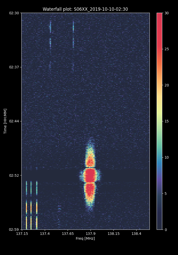
To get a quick preview of the raw RF data, we create waterfall plots. Creates a waterfall plot of sample data provided with EMBERS using
the single_waterfall() function with the waterfall_single cli tool:
$ waterfall_single
>>> Waterfall plot saved to ./embers_out/rf_tools/S06XX_2019-10-10-02:30.png
Or using single_waterfall() as shown in the example below:
from pathlib import Path
from embers.rf_tools.rf_data import single_waterfall

rf_file = "tiles_data/S06XX/2019-10-10/S06XX_2019-10-10-02:30.txt"
out_dir  = "embers_out/rf_tools"

print(f"Waterfall plot saved to ./{out_dir}/{Path(rf_file).stem}.png")
single_waterfall(rf_file, out_dir)
We can also create a set of waterfall plots for all rf_files within a date interval using the waterfall_batch() function, with
either the provided cli tool or with the following example code
$ waterfall_batch
>>> Processing rf data files between 2019-10-10 and 2019-10-10
>>> Saving waterfall plots to: ./embers_out/rf_tools/waterfalls
from embers.rf_tools.rf_data import waterfall_batch

data_dir = "./tiles_data"
start_date = "2019-10-10"
stop_date = "2019-10-10"
out_dir  = "embers_out/rf_tools"

print(f"Processing rf data files between {start_date} and {stop_date}")
print(f"Saving waterfall plots to: ./{log_dir}")
waterfall_batch(start_date, stop_date, data_dir, out_dir)
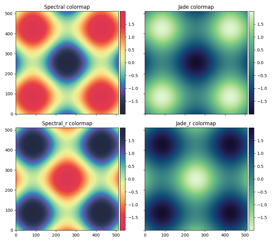
Colormaps
EMBERS comes with two beautiful custom colormaps called spectral & jade. The spectral colormap is non-linear and is just used to
visualise raw data and maximize dynamic range, while jade is perceptually uniform and sequential and is suitable for science.
To get a preview of how amazing they are
$ colormaps
>>> Plot of embers colormaps saved to ./embers_out/rf_tools/colormaps.pngy
from embers.rf_tools.colormaps import plt_colormaps, jade, spectral

spec, spec_r = spectral()
jade, jade_r = jade()
out_dir="./embers_out/rf_tools"

plt_colormaps(spec, spec_r, jade, jade_r, out_dir)
print(f"Plot of embers colormaps saved to {out_dir}/colormaps.pngy")
Align Data
The RF Explorers used to record satellite data may not record data at exactly the same frequency and may not start recording at exactly the same time. In fact, the older models record at approximately 6 Hz, while the newer ones are capable of a sampling rate of nearly 9 Hz. This discrepency in sampling rates makes it difficult to compare any two data samples. This issue is overcome by smoothing the data, along the time axis, with a Savitzky-Golay filter. Interpolating the smoothed data and resampling it at a constant frequency [ 1 Hz ] gives us a easier data set to work with.
Two level of savgol filters are applied, first to capture deep nulls + small structure, and second level to smooth over noise. A cli tool align_single,
based on the plot_savgol_interp() function,
can be used to play with the various parameters available. Sensible defaults are provided as a starting point. The following code plots one frequency channel of
RF data and shows the efficacy of the selected smoothing filter.
$ align_single
>>> Saving sample savgol_interp plot to: ./embers_out/rf_tools/savgol_interp_sample.png
Alternately, the following sample code may be used to achieve identical results:
from embers.rf_tools.align_data import plot_savgol_interp

ref_file="tiles_data/rf0XX/2019-10-10/rf0XX_2019-10-10-02:30.txt"
tile_file="tiles_data/S06XX/2019-10-10/S06XX_2019-10-10-02:30.txt"
savgol_window_1=11
savgol_window_2=15
polyorder=2
interp_type="cubic"
interp_freq=1
channel=59
out_dir="./embers_out/rf_tools"


plot_savgol_interp(
    ref=ref_file,
    tile=tile_file,
    savgol_window_1=savgol_window_1,
    savgol_window_2=savgol_window_2,
    polyorder=polyorder,
    interp_type=interp_type,
    interp_freq=interp_freq,
    channel=channel,
    out_dir=out_dir,
)

print(f"Saving sample savgol_interp plot to: {out_dir}/savgol_interp_sample.png")

We can now align all the raw RF files within a date interval using the align_batch() function. Every pair of reference and
MWA tile are smoothed and aligned and saved to compressed npz file by savez_compressed().
WARNING: This is probably the most resource hungry section. It typically took me 2 days to process 5 months of data, on a machine with 40 cpu cores. Beware, and be patient.
The --max_cores option is available to limit number of cores used by the align_batch paralelized cli-tool. If you are experimenting with EMBERS
on a laptop it is highly suggested that you use set --max_cores=1 for any batch script. This is sufficent for testing and will not run your laptop to the
ground by using all availible resources. An analysis of the performance of this tool can be found at Performance.
The align_batch cli tool is a convenient way to align large volumes of data
$ align_batch
>>> Aligned files saved to: ./embers_out/rf_tools/align_data
Alternately, the following sample code may be used to achieve identical results:
from embers.rf_tools.align_data import align_batch

start_date="2019-10-10"
stop_date="2019-10-10"
savgol_window_1=11
savgol_window_2=15
polyorder=2
interp_type="cubic"
interp_freq=1
data_dir = "./tiles_data"
out_dir="./embers_out/rf_tools"


align_batch(
    start_date=start_date,
    stop_date=stop_date,
    savgol_window_1=savgol_window_1,
    savgol_window_2=savgol_window_2,
    polyorder=polyorder,
    interp_type=interp_type,
    interp_freq=interp_freq,
    data_dir=data_dir,
    out_dir=out_dir,
)
print(f"Aligned files saved to: {out_dir}")
Sat Utils
embers.sat_utils is used to compute various satellite orbital parameters. Outputs of this module are saved to the ./embers_out/sat_utils directory.
Ephemeris data of satellites active in the 137 - 139 MHz frequency window are available at Space-Track.org in the form of TLE files, which can be downloaded. The satellites used in this analysis are the ORBCOMM communication satellites and the NOAA & METEOR weather satellites.
Download Ephemeris
Warning
To download TLEs from Space-Track.org, make an account and obtain login credentials.
Once valid login credentials have been obtained, download tle files with the download_tle() using the following cli tool
$ download_tle --start_date=YYYY-MM-DD --stop_date=YYYY-MM-DD --st_ident=** --st_pass=**
>>> TLE files saved to ./embers_out/sat_utils/TLE
or with the following example script
from embers.sat_utils.sat_list import download_tle, norad_ids


start_date = "2019-10-01"
stop_date = "2019-10-10"
out_dir = "./embers_out/sat_utils/TLE"
n_ids = norad_ids()

# Make account on space-track.org and enter credentials below
st_ident = "test@user.com"
st_pass = "*******"

download_tle(
    start_date,
    stop_date,
    n_ids,
    st_ident=st_ident,
    st_pass=st_pass,
    out_dir=out_dir,
)

print(f"TLE files saved to {out_dir}")
Satellite ephemeris
The downloaded TLE files must be parsed and analysed before they make any sense. A python package called skyfield and it’s
EarthSatellite class were invaluable for this, enabling
the computation of satellites trajectories over a geographical location (MWA telescope). Sample TLE data can be analysed and a sky coverage plot created with
the save_ephem() with either the following cli tool or the equivalent sample code.
$ ephem_single
>>> Saved sky coverage plot of satellite [25417] to ./embers_out/sat_utils/ephem_plots/25417.png
>>> Saved ephemeris of satellite [25417] to ./embers_out/sat_utils/ephem_data/25417.npz
from pathlib import Path
from embers.sat_utils.sat_ephemeris import save_ephem

sat="25417"
tle_dir="./embers_out/sat_utils/TLE"
cadence = 4
location = (-26.703319, 116.670815, 337.83)
out_dir = "./embers_out/sat_utils/"

status = save_ephem(sat_name, tle_dir, cadence, location, out_dir)
print(status)

Analysing a batch of TLE files is achieved with the ephem_batch() function, which converts the TLE files downloaded with
download_tle into satellite ephemeris data: rise time, set time, alt/az arrays at a given time cadence. This is saved to a npz file which will be used
to plot the satellite sky coverage over the geographic location supplied. It can be used with the following cli tool
The --max_cores option is available to limit number of cores used by the ephem_batch paralelized cli-tool below.
$ ephem_batch
>>> Saving logs to ./embers_out/sat_utils/ephem_data
>>> Saving sky coverage plots to ./embers_out/sat_utils/ephem_plots
>>> Saving ephemeris of satellites to ./embers_out/sat_utils/ephem_data
or with the equivalent example script
from embers.sat_utils.sat_ephemeris import ephem_batch

cadence = 4
out_dir = "./embers_out/sat_utils/"
tle_dir = "./embers_out/sat_utils/TLE"
location = (-26.703319, 116.670815, 337.83)

ephem_batch(tle_dir, cadence, location, out_dir)
Chronological ephemeris
Collate ephemeris data generated above by ephem_single or ephem_batch for multiple satellites and determine all satellites present in each
30 minute observation and what their trajectories at the geographic location. The save_chrono_ephem() function saves
chronological ephemeris data to json files in ./embers_out/sat_utils/ephem_chrono.
Use the following cli tool to collate satellite data
$ ephem_chrono
>>> Saving chronological Ephem files to: ./embers_out/sat_utils/ephem_chrono
>>> Grab a coffee, this may take more than a couple of minutes!
or the equivalent sample script
from embers.sat_utils.chrono_ephem import save_chrono_ephem

time_zone = "Australia/Perth"
start_date = "2019-10-10"
stop_date = "2019-10-10"
interp_type = "cubic"
interp_freq = 1
ephem_dir = "./embers_out/sat_utils/ephem_data"
out_dir = "./embers_out/sat_utils/ephem_chrono"

save_chrono_ephem(
    time_zone,
    start_date,
    stop_date,
    interp_type,
    interp_freq,
    ephem_dir,
    out_dir,
)
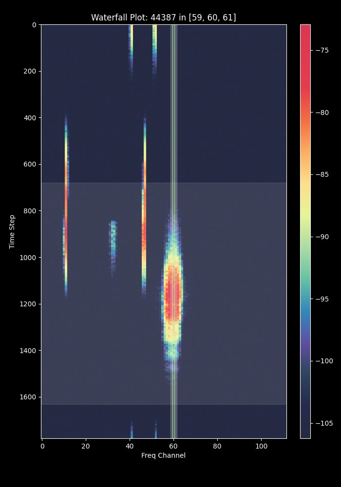
Satellite Channels
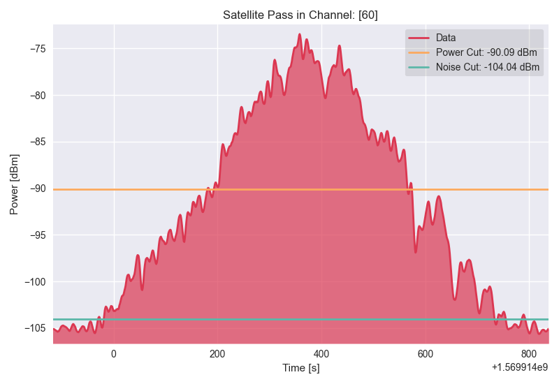
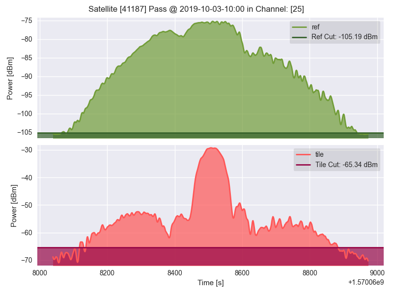
As access to the ORBCOMM interface box is not readily available, the channels in which each satellite transimits can be determined with a careful analysis of the RF data and satellite ephemeris. We use reference data to detect satellite channels because it has the best SNR. Pairing a reference RF data file, with it’s corresponding chrono_ephem.json file gives us the satellite expected within each 30 minute observation. Looping over the satellites in the chrono_ephem files, we identify the temporal region of the rf data where we expect to see its signal. We now use a series of thresholding criteria to help identify the most probable channel. The following thresholds were used to identify the correct channel:
Noise threshold
A Noise floor of the RF data array is determined by using a standard deviation (σ) -threshold. We define a satellite theshold called s. If a channel of
the RF data array has power exceeding s•σ, it is masked out. By default, σ=1, which means that any channel with power exceeding one std above the median
power are excluded. The median power of the remaining data is called μ_noise. The median absolute deviation (MAD) of the remaining data is called
σ_noise. We now defile a noise floor of the RF data array, based on a noise theshold denoted by n, which defaults to 3.
noise floor = μ_noise + n•σ_noise
Now, any power in the RF data array, exceeding the noise floor is a satellite candidate.
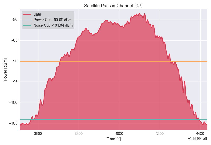
Power threshold
We also expect the peak power of a satellite signal to exceed a certain theshold. By default this is set to 5 dB above the noise floor.
Window Occupancy
Satellite ephemeris data tells us when we expect to see a satellite in the sky, at a given geographic location. We use this to define a temporal window within
the RF data array, and search for the satellite within it. We look for RF signals, above the noise floor, which occupy more than a given fraction of the
window, and less than 100%. By default the window occupancy is defined as follows, but the lower limit may be changed
0.8 ≤ window occupancy ≤ 1.0
The analysis discusses above is implemented with the batch_window_map() function. Satellite channels can be identified with
the sat_channels cli tool:
The --max_cores option is available to limit number of cores used by the sat_channels paralelized cli-tool below.
$ sat_channels
>>> Window channel maps will be saved to: ./embers_out/sat_utils/sat_channels
or the sample script below:
from embers.sat_utils.sat_channels import batch_window_map

start_date = "2019-10-10"
stop_date = "2019-10-10"
ali_dir = "./embers_out/rf_tools/align_data"
chrono_dir = "./embers_out/sat_utils/ephem_chrono"
sat_thresh = 1
noi_thresh = 3
pow_thresh = 15
occ_thresh = 0.80
out_dir = "./embers_out/sat_utils/sat_channels"
plots = True

batch_window_map(
    start_date,
    stop_date,
    ali_dir,
    chrono_dir,
    sat_thresh,
    noi_thresh,
    pow_thresh,
    occ_thresh,
    out_dir,
    plots=plots,
)
In the following waterfall plots, the horizontal highlighted band represents the temporal window, while the vertical highlighted channels represent possible identified channels. The green vertical channel represents the most probable channel.

The plots below represent the power in the selected channel, with various thresholds displayed
Finally, an ephemeris plot of the trajectories of the two satellites identified

MWA Utils
embers.mwa_utils is used to download and metadata of the MWA Telescope and compute FEE beam models. Outputs of this
module are saved to ./embers_out/mwa_utils. The MWA telescope is electronically pointed using delay-line beam-formers. Metadata regarding the pointing
of the telescope at various times and the health of dipoles that make up the MWA tiles can be obtained from metadata created by the telescope.
MWA Pointings
Download MWA metadata and determine the pointings of the telescope during each 30 minute rf observation. Before we download the metadata, we have a couple of hoops to jump through.
MWA metadata is downloaded in json format, from website. Each webpage can contain a maximum of 200 entries. We need to visit ws.mwatelescope.org/metadata/find and determine the number of pages required to download all metadata within a date interval.
On the site, enter the start and stop date, change the page size to 200 and click search. Note down the number of pages returned by the search.
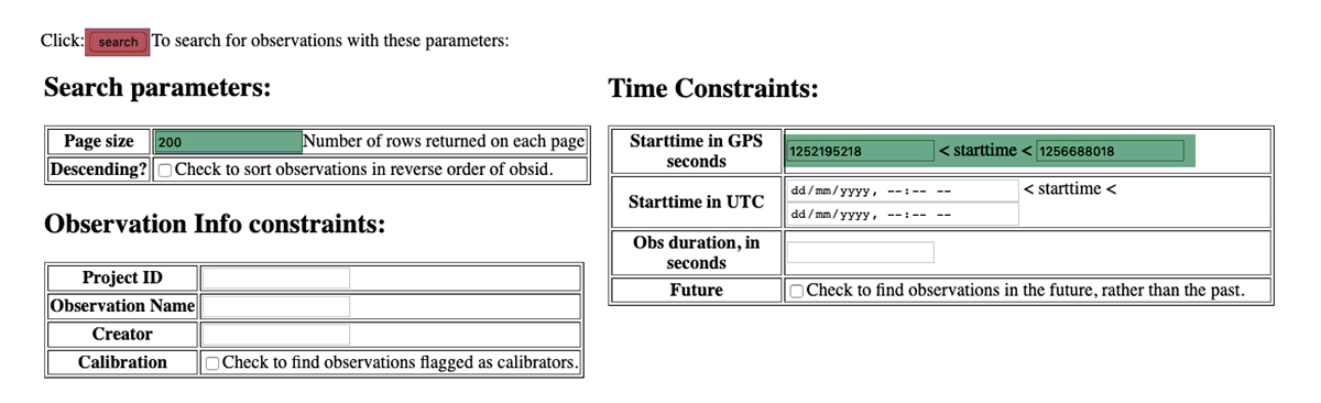

We now know that we need to download 74 pages of metadata, which can be done using the mwa_point_meta() function with
either the following cli tool or the sample script
$ mwa_pointings
>>> Downloading MWA metadata
>>> Due to download limits, this will take a while
>>> ETA: Approximately 0H:01M
>>> MWA tile pointing data saved to ./embers_out/mwa_utils
from embers.mwa_utils.mwa_pointings import mwa_point_meta

start_date = "2019-10-09"
stop_date = "2019-10-11"
num_pages = 4
time_thresh = 1
time_zone = "Australia/Perth"
rf_dir = "./tiles_data"
out_dir = "./embers_out/mwa_utils"

mwa_point_meta(
    start_date, stop_date, num_pages, time_thresh, time_zone, rf_dir, out_dir
)
print(f"MWA tile pointing data saved to {out_dir}")
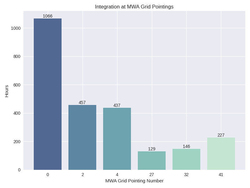
This process can take up to a couple of hours due to network limits on frequency of downloads from the MWA servers. A file called obs_pointing.json will be created which contains all 30 minute observations with more than a 60% majority of time at a single pointing. A histogram showing maximum theoretical integration times per pointing is created. This limit is often not achieved due to pointings changing during 30 minute observations and equipment malfunctions. By checking to see if corresponding RF raw data files exist for given observation times, a plot of actual integration time for each tile is generated.
The following plots contain data from ~6 months between 2019-09-12 and 2020-03-16.

MWA Dipoles
MWA metadata can also tell us if dipoles in the tiles which have been used are not functional. We can check this using the
mwa_flagged_dipoles() function with the following cli tool or example script
$ mwa_dipoles
>>> Downloading MWA metafits files
>>> Due to download limits, this will take a while
>>> ETA: Approximately 0H:06M
>>> MWA dipole flagging data saved to ./embers_out/mwa_utils
from embers.mwa_utils.mwa_dipoles import mwa_flagged_dipoles

num_files = 14
out_dir = "./embers_out/mwa_utils"

mwa_flagged_dipoles(num_files, out_dir)
print(f"MWA dipole flagging data saved to {out_dir}")
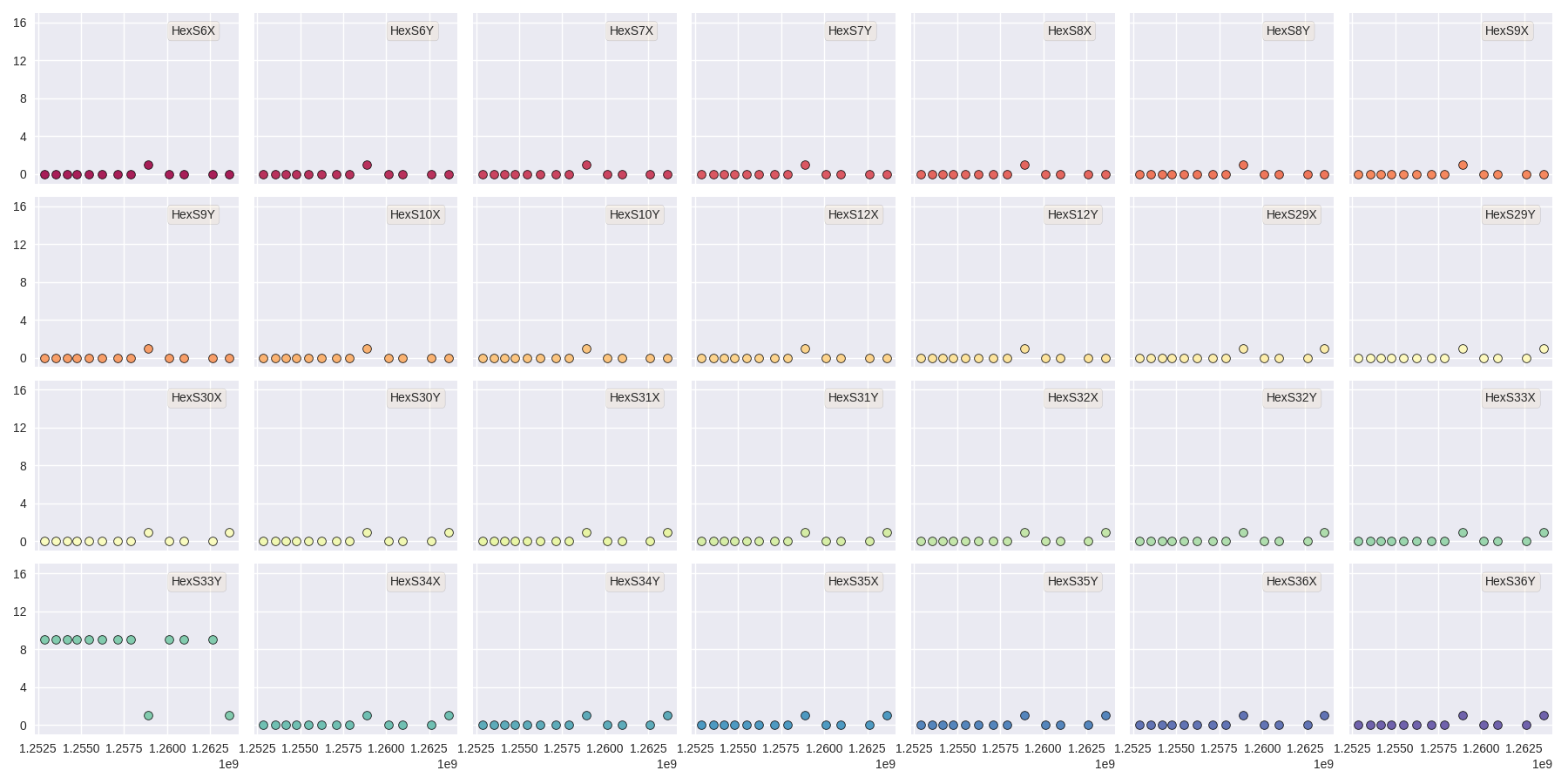
The above figure show us that tile S33YY had its 9th dipole flagged for most of the duration of the observational period.
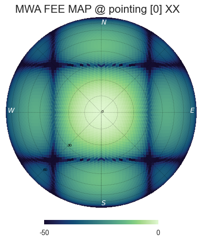
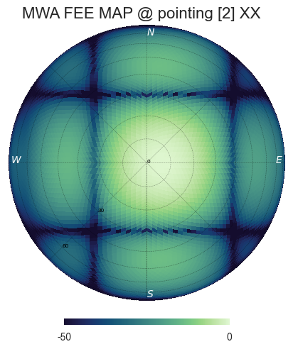
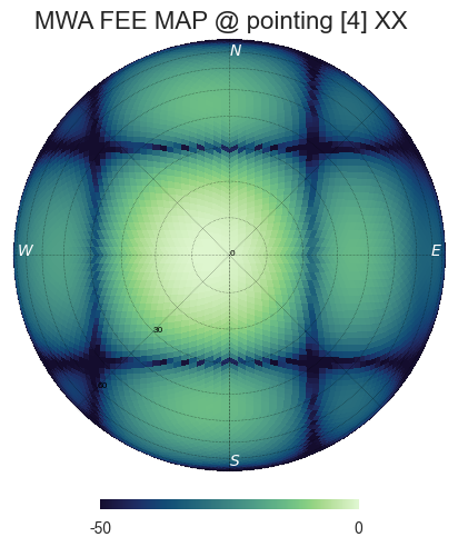
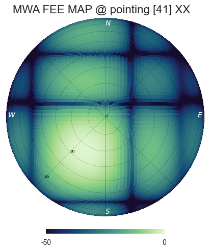
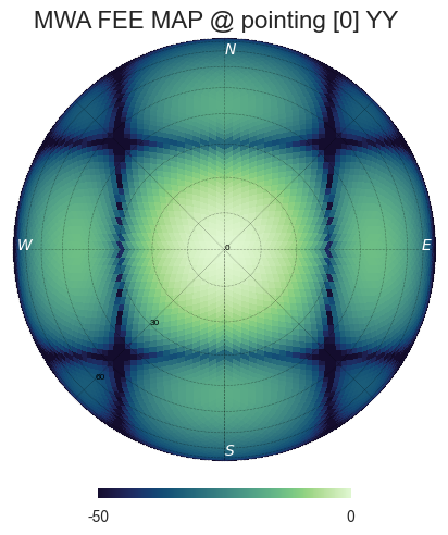
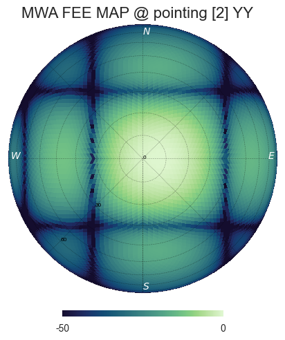
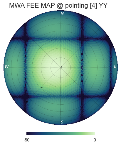
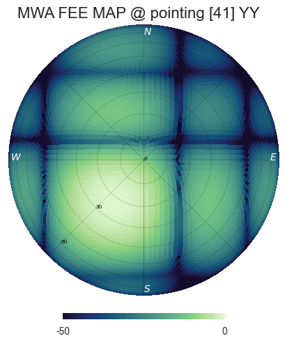
MWA FEE
MWA Fully Embedded Element (FEE) beam models represent the cutting edge of simulated MWA beam models. We generate MWA FEE model healpix maps at the given nside
using the MWA Primay Beam GitHub repository and the mwa_fee_model() function, with
the following mwa_fee cli tool of example script
$ mwa_fee
>>> MWA_FEE maps saved to: ./embers_out/mwa_utils
from embers.mwa_utils.mwa_fee import mwa_fee_model

# Healpix nside
nside = 32

# List of MWA pointings at which to evaluate the beam
pts = "0, 2, 4, 41"
pointings = [int(item) for item in pts.split(',')]

# List of flagged dipoles with indices from 1 to 32
# 1-16 are dipoles of XX pol while 17-32 are for YY
# 0 == No flagged dipoles
fgs = "0"
flags = [int(item) for item in _args.flags.split(',') if not "0"]

out_dir = "./embers_out/mwa_utils"

mwa_fee_model(out_dir, nside, pointings, flags)
print(f"MWA_FEE maps saved to: {out_dir}")
Tile Maps
There be magic here. We can finally make beam maps of the MWA tiles!
embers.tile_maps is used to create tile maps by aggregating satellite data. Outputs of this module are saved to ./embers_out/tile_maps
Ref Models
Convert FEKO models on the reference antennas into usable healpix maps using the ref_healpix_save() function.
These maps will later be used to remove effects introduced by satellite beam shapes. Use the ref_models cli tool or the following sample code.
$ ref_models
>>> Reference models saved to: ./embers_out/tile_maps/ref_models
from embers.tile_maps.ref_fee_healpix import ref_healpix_save

nside = 32
out_dir = "./embers_out/tile_maps/ref_models"

ref_healpix_save(_nside, _out_dir)

RFE Calibration
Calibrate non-linear gains of RF Explorers at high powers by comparing satellite rf data to corresponding slices of the MWA FEE model.
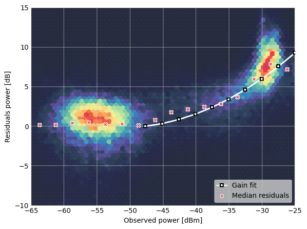
It was observed that the RF explorers enter a non-linear gain regime at high input powers, leading to a deficit in recorded power. In this section we aim to solve for a global gain calibration solution which can be applied to all data recorded by the RF Explorers, recovering the missing power. This non-linear effects were only observed for RF Explorers connected to the MWA tiles and not the reference antennas.
To first order, we presume that the FEE models of the MWA beam are a good representation of reality. The RF explorers were set to be sensitive to power in the range of -120 dBm to +5 dBm. We observe a “flattening” of the RF Explorer response when powers exceed -50 dBm. To characterise this we compute a MWA beam slice, for every satellite pass, using eq (1) from the paper.
MWA = (tile/ref)•ref_fee
The MWA beam profile is the ratio of tile and reference power, multiplied by the reference FEE model. The MWA beam profile is then scaled back down to the power of the original tile data, using a single multiplicative gain factor, determined using a chi-squared minimization. We now compare the scaled mwa slice to a corresponding slice of the MWA FEE beam model. This tells us where there is missing power. We record the observed power and the residual power between the scaled MWA slice and the FEE model. By repeatings this process for all satellite passes observed, we build up a distribution of residual power, which can be fit by a low order polymonial. This polynomial is the global calibration solution of the non-linear RF Explorer gain, which can be applied to data in the next step.
Determine the RF Explorer gain calibration solution using the rfe_batch_cali() function with the rfe_calibration
cli tool or the following sample script
The --max_cores option is available to limit number of cores used by the rfe_calibration paralelized cli-tool below.
$ rfe_calibration
>>> RF Explorer calibration files saved to: ./embers_out/tile_maps/rfe_calibration
from embers.tile_maps.tile_maps import rfe_batch_cali

start_date="2019-10-10"
stop_date="2019-10-10"

# Power at which RFE gain variations begin
start_gain = -50

# Power at which RFE gain variations saturate
stop_gain = -30

# σ threshold to detect sats in the computation of rf data noise_floor
sat_thresh = 1

# noise threshold: multiples of mad
noi_thresh = 3

# Peak power which must be exceeded for satellite pass to be considered
pow_thresh = 5

# Path to reference feko model
ref_model = "embers_out/tile_maps/ref_models/ref_dipole_models.npz"

# Path to MWA FEE model
fee_map = "embers_out/mwa_utils/mwa_fee/mwa_fee_beam.npz"

# Healpix Nside
nside = 32

# Path to obs_pointings.json
obs_point_json = "embers_out/mwa_utils/obs_pointings.json"

# Directory where aligned rf data lives
align_dir = "embers_out/rf_tools/align_data"

# Directory where Chronological satellite ephemeris data lives
chrono_dir = "embers_out/sat_utils/ephem_chrono"

# Directory where satellite frequency channel maps are saved
chan_map_dir = "embers_out/sat_utils/sat_channels/window_maps"

# Directory where RF Explorer calibration data will be saved
out_dir = "./embers_out/tile_maps/rfe_calibration"

rfe_batch_cali(
    start_date,
    stop_date,
    start_gain,
    stop_gain,
    sat_thresh,
    noi_thresh,
    pow_thresh,
    ref_model,
    fee_map,
    nside,
    obs_point_json,
    align_dir,
    chrono_dir,
    chan_map_dir,
    out_dir,
)
The following plot represents RF Explorer gain calibration using 6 months of data
Tile Maps
Batch process satellite RF data to create MWA beam maps and intermediate plots.
As in the previous section, satellite data is gridded onto a healpix map based on ephemeris trajectories in the sky. The data from the MWA tiles is corrected
using the RF Explorer gain calibration solution formed in the perevious section. A couple of different types of data products are created using the
tile_maps_batch() with the tile_maps cli tool or the following sample script
The --max_cores option is available to limit number of cores used by the tile_maps paralelized cli-tool below.
$ tile_maps --start_date=2019-10-10 --stop_date=2019-10-10 --plots=True
>>> MWA tile map files saved to: ./embers_out/tile_maps/tile_maps
from embers.tile_maps.tile_maps import tile_maps_batch

start_date="2019-10-10"
stop_date="2019-10-10"

# σ threshold to detect sats in the computation of rf data noise_floor
sat_thresh = 1

# noise threshold: multiples of mad
noi_thresh = 3

# Peak power which must be exceeded for satellite pass to be considered
pow_thresh = 5

# Path to reference feko model
ref_model = "embers_out/tile_maps/ref_models/ref_dipole_models.npz"

# Path to MWA FEE model
fee_map = "embers_out/mwa_utils/mwa_fee/mwa_fee_beam.npz"

# Path to RF Explorer gain calibration solution
rfe_cali = "embers_out/tile_maps/rfe_calibration/rfe_gain_fit.npy"

# Healpix Nside
nside = 32

# Path to obs_pointings.json
obs_point_json = "embers_out/mwa_utils/obs_pointings.json"

# Directory where aligned rf data lives
align_dir = "embers_out/rf_tools/align_data"

# Directory where Chronological satellite ephemeris data lives
chrono_dir = "embers_out/sat_utils/ephem_chrono"

# Directory where satellite frequency channel maps are saved
chan_map_dir = "embers_out/sat_utils/sat_channels/window_maps"

# Directory where RF Explorer calibration data will be saved
out_dir = "./embers_out/tile_maps/rfe_calibration"

# If True, create a zillion diagnostic plots at the project_tile_healpix stage
plots = True

# Turn RFE calibration on or off. Default=True.
rfe_cali_bool = True

tile_maps_batch(
    start_date,
    stop_date,
    sat_thresh,
    noi_thresh,
    pow_thresh,
    ref_model,
    fee_map,
    rfe_cali,
    nside,
    obs_point_json,
    align_dir,
    chrono_dir,
    chan_map_dir,
    out_dir,
    plots,
    rfe_cali_bool,
)
Tile Maps Raw
For each satellite pass recorded by the MWA tiles and reference antennas, apply equation (1) from the beam paper to remove
satellite beam effect and calculate a resultant cross-sectional slice of the MWA beam. Using satellite ephemeris data, project
this beam slice onto a healpix map. This function also applies RFE gain correction using the gain solution created by
rfe_collate_cali(). The resulting healpix map is saved to a .npz file in
with the data structured in nested dictionaries, which have the following structure.
map*.npz
├── mwa_map
│   └── pointings
│       └── satellites
│           └── healpix maps
├── ref_map
│   └── pointings
│       └── satellites
│           └── healpix maps
├── tile_map
│   └── pointings
│       └── satellites
│           └── healpix maps
└── time_map
    └── pointings
        └── satellites
            └── healpix maps
The highest level dictionary contains normalized mwa, reference, tile and time maps. Within each of these, there are dictionaries for each of the telescope pointings:0, 2, 4, 41. Within which there are dictionaries for each satellite norad ID, which contain a healpix map of data from one satellite, in one pointing. This structure may seem complicated, but is very useful for diagnostic purposes, and determining where errors in the final tile maps come from. The time maps contain the times of every data point added to the above maps.
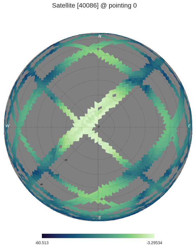
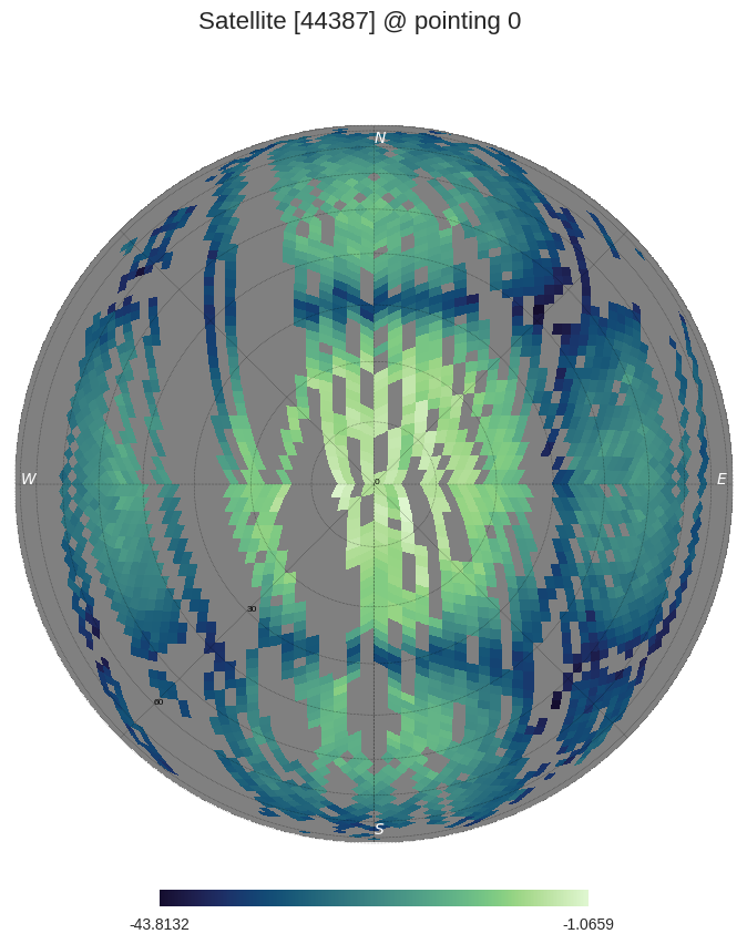
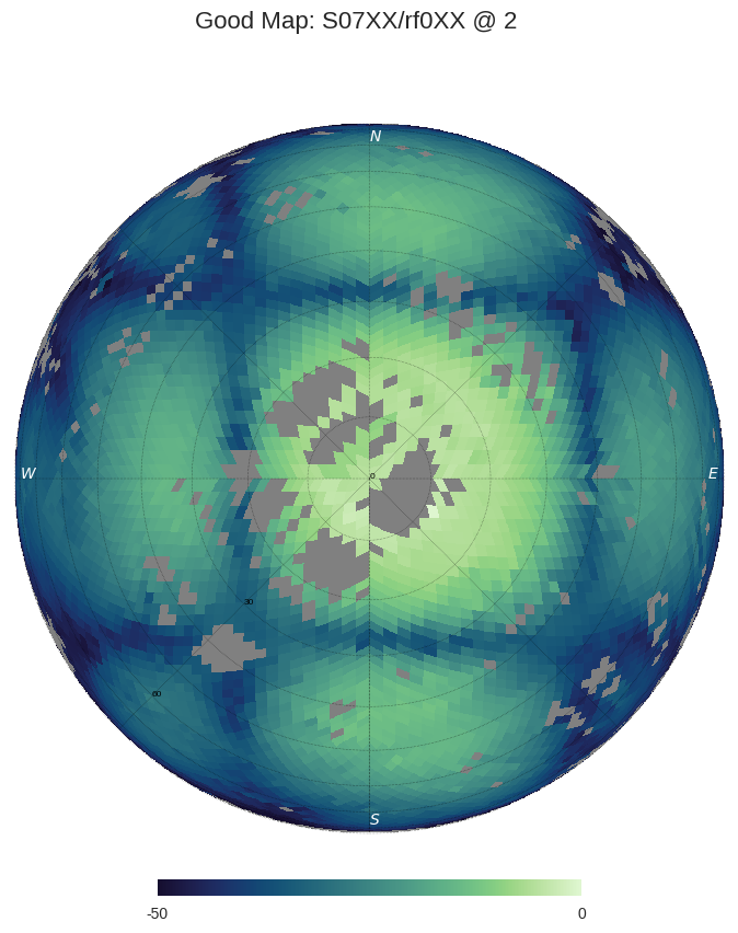
Sat Plots
Using the raw tile maps generated above, we can plot sky coverage maps for each of the 72 satellites used. This proccess was extremely useful in showing us
that most of the 72 selected satellites are out of the frequnecy window of this experiment. This is seen by extremely sparce sky coverage for satellite data
collected over the course of 6 months, which strongly suggests that the few passes identifies in these sparce satellite maps must be misidentifications
at the satellite channels stage of processing. We use these maps to select 18 good satellites which have excellent sky coverage.

For further processing, we restrict our maps to data from the 18 good satellite, which significantly improves the quality of the beam maps by excluding spurious misidentified signals.
We also plot profiles of each satellite pass to see how effective the RF Explorer gain calibration is and also implement a p-value goodness of fit test, which is used to filter out the last couple of bad signals which have persisted. This filter is set to a very conservative value, only rejecting satellite passes which are completely different from corresponding slices of the MWA FEE beam.
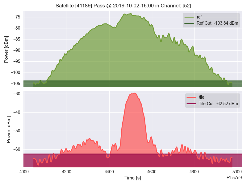
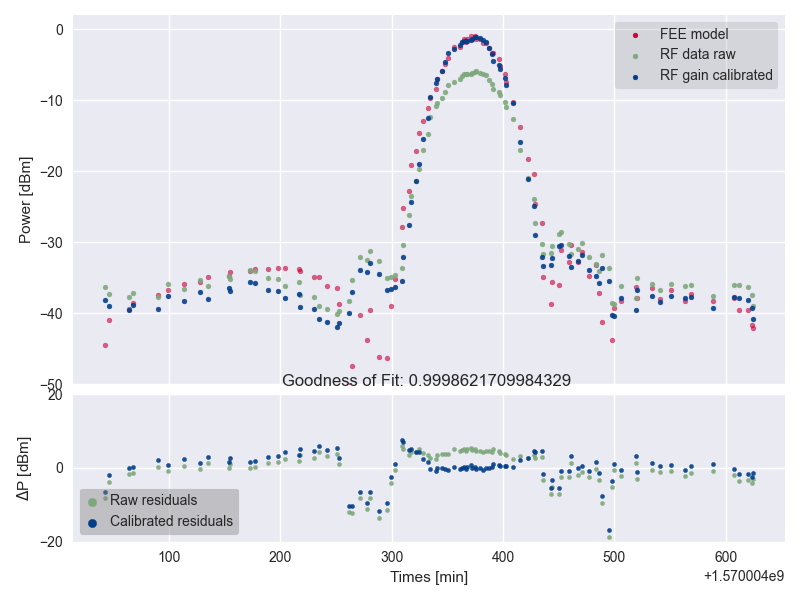
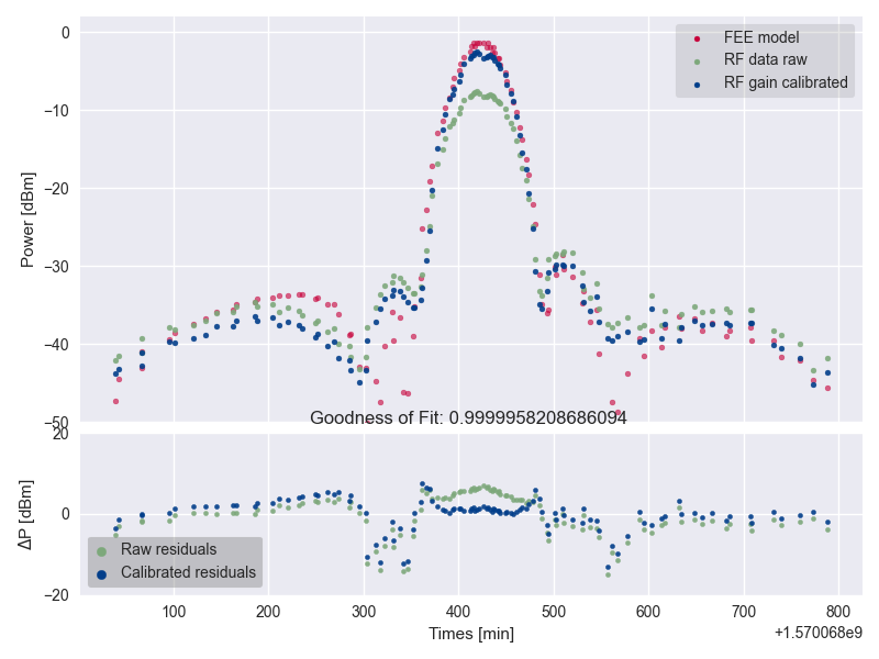
The upper two pannels show the tile and reference RF power profiles for two satellite passes. The latter two panels display the raw tile data in green, with the blue data indicating RF gain corrected tile data. The crimson data is a corresponding slice of the MWA FEE model, and shows good agreement with the corrected (blue) tile data.
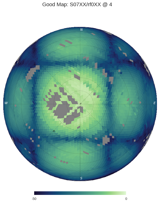
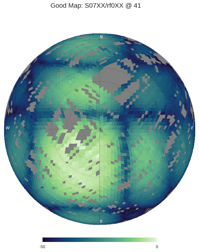
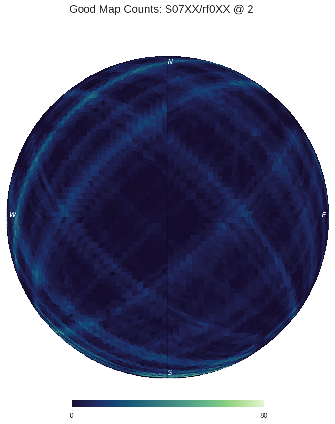
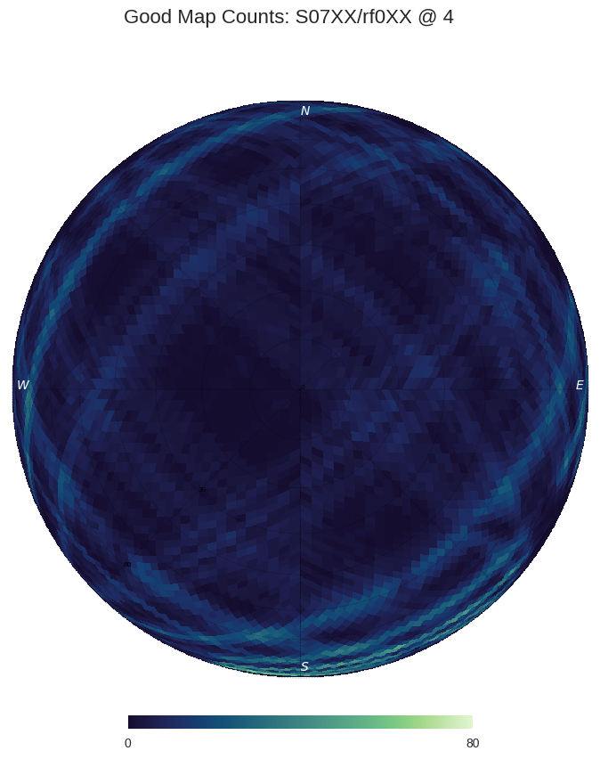
Tile Maps Clean
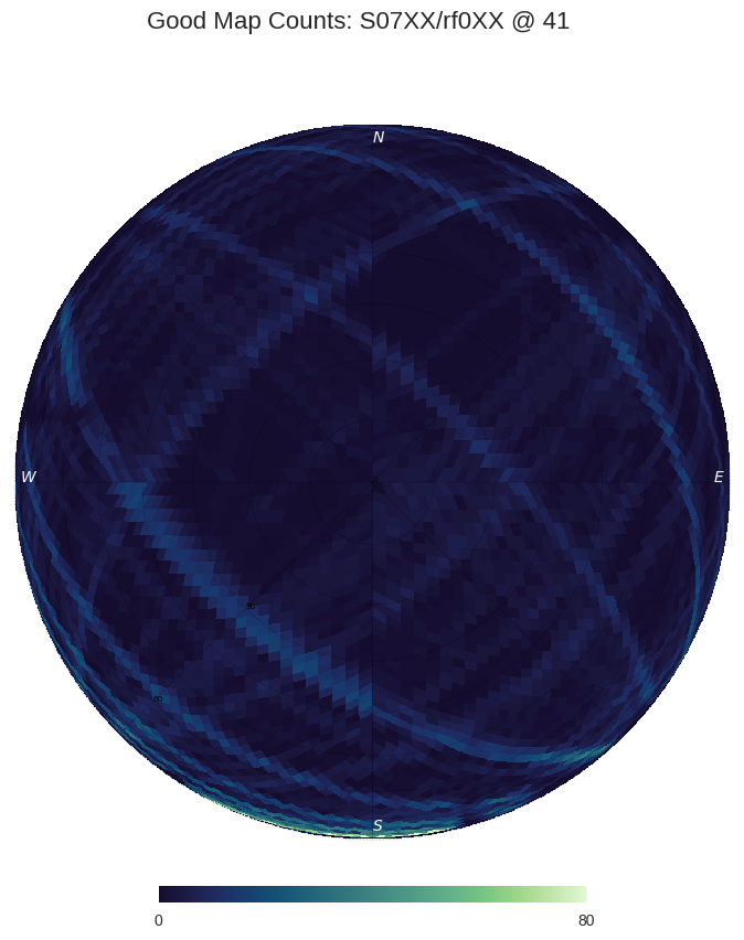
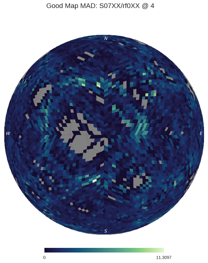
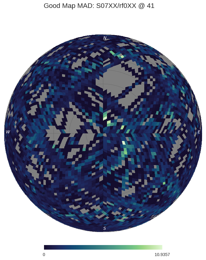
We now form clean MWA beam maps at all four pointings (0, 2, 4, 41), using the 18 good satellites. The first row of images are MWA beam maps, the second row are satellite pass counts in each pixel while the third row are errors on each pixel.


Null Test
The two reference antennas provide the ability to perform a null test, in which we compare the performance of each refrerence antenna against each other using
the null_test() function. This can be achieved using the null_test cli tool or the following sample script
$ null_test
>>> Null tests saved to embers_out/tile_maps/null_test
from embers.tile_maps.null_test import null_test

# Healpix Nside
nside = 32

# Maximum zenith angle upto which to perform the null test
za_max = 90

# Reference feko healpix model created by embers.tile_maps.ref_fee_healpix
ref_model = "embers_out/tile_maps/ref_models/ref_dipole_models.npz"

# Directory with tile_maps_raw, created by embers.tile_maps.tile_maps.project_tile_healpix
map_dir = "embers_out/tile_maps/tile_maps/tile_maps_raw"

# Dir where null tests will be saved
out_dir = "./embers_out/tile_maps/null_test"

null_test(
    nside,
    za_max,
    ref_model,
    map_dir,
    out_dir
)
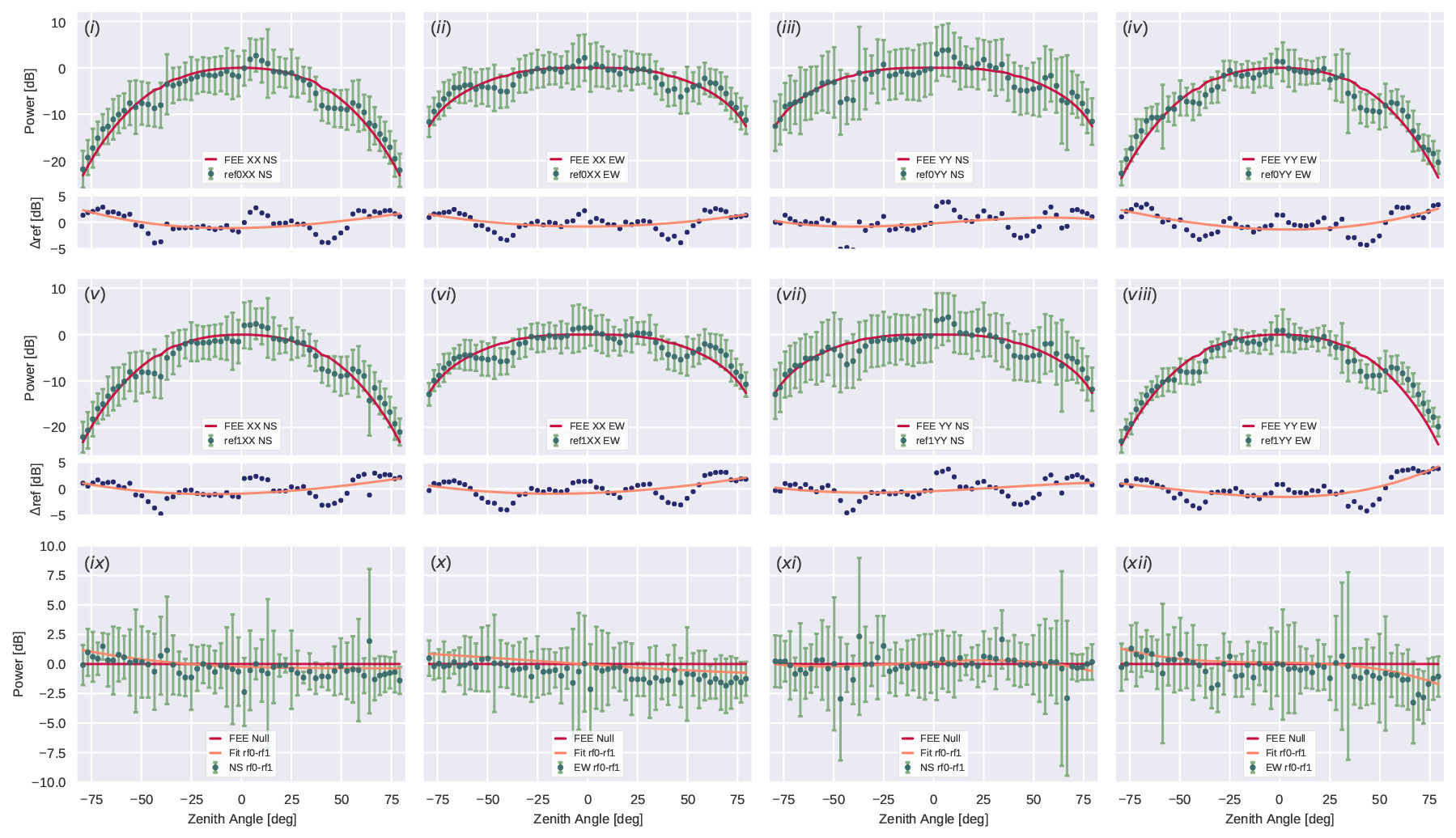
The first two rows represent slices of the measured reference beam pattern, compared to the FEKO reference beam model. The last row compares corresponding slices of two reference maps against each other.
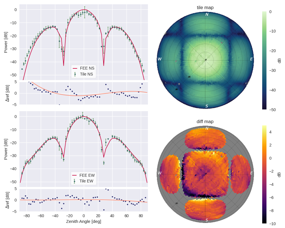
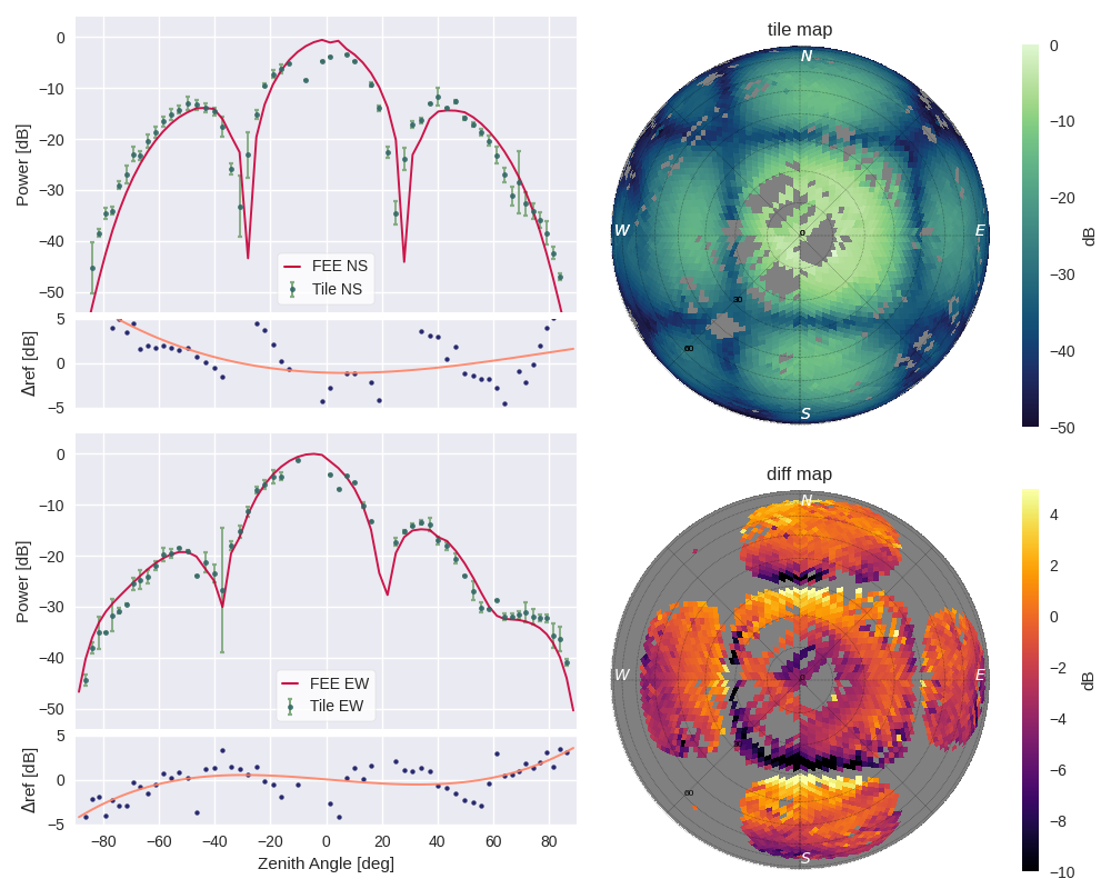
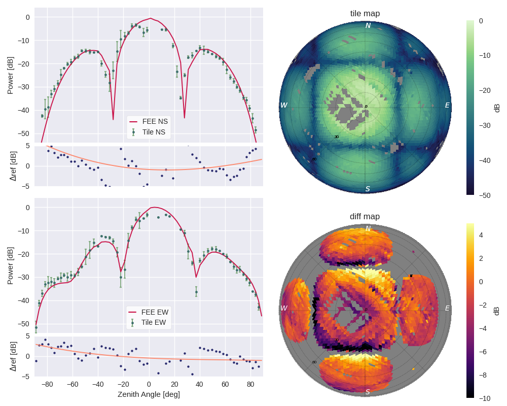
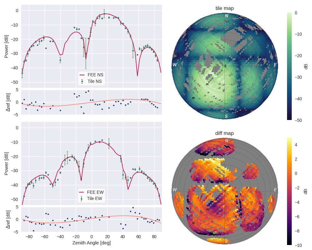
Compare Beams
Compare measured MWA beam maps created above, with MWA FEE models using the batch_compare_beam() function with the
compare_beams cli tool or the following sample script
The --max_cores option is available to limit number of cores used by the compare_beams paralelized cli-tool below.
$ compare_beams
>>> Beam comparison plots saved to: ./embers_out/tile_maps/compare_beams
from embers.tile_maps.compare_beams import batch_compare_beam

# Healpix Nside
nside=32

# MWA FEE healpix model created by embers.mwa_utils.mwa_fee
fee_map = "embers_out/mwa_utils/mwa_fee/mwa_fee_beam.npz"

# Directory with tile_maps_clean, created by embers.tile_maps.tile_maps.mwa_clean_maps
map_dir = "embers_out/tile_maps/tile_maps/tile_maps_clean"

# Dir where beam comparison plots will be saved
out_dir = "./embers_out/tile_maps/compare_beams"

batch_compare_beam(
    nside,
    fee_map,
    map_dir,
    out_dir
)
Testing EMBERS
EMBERS comes with a set of automated tests which can be run. To do this, install EMBERS from the github repository, install the necessary python dependancies and follow the installations below.
git clone https://github.com/amanchokshi/EMBERS.git
cd EMBERS

# Setup a virtual enviroment
python -m venv embers-env
source embers-env/bin/activate

pip install .
pip install -r requirements_dev.txt

# Run automated tests
pytest